In this post we are going to talk about how to quickly and easily analyze data with Python. Specifically this will show you how to import and export data from CSV’s (comma seperated variables) into Python. Note that this post is a work in progress and information will continue to be updated.
Click here to view the presentation slides. They have some useful links to documentation that can help you in your Python endeavours!
a = 1
b = 2
a + b
3
a - b
-1
a * b
2
b / a
2.0
b % a
0
a = 2
b = 3
b**a
9
for i in range(0, 10, 1):
    print(i)
0
1
2
3
4
5
6
7
8
9
NOTE THAT THE LOOP DOES NOT PRINT 10
Some functionality isnt supported by Python by default. Common libraries include:
Read more about Python internal libraries here
You can import an entire library under an shortened alias. The following are the typical conventions:
import numpy as np
import pandas as pd
import matplotlib as plt
Say I have a list of items in Python. The following are helpful indexing conventions. Read more about lists here
sample_list = [1, 2, 3, 4, 5]
sample_list[0]
1
sample_list[-1]
5
sample_list.pop(0)
1
sample_list
[2, 3, 4, 5]
for item in sample_list:
    print("The item {} multiplied by 2 is {}".format(item, item*2))
The item 2 multiplied by 2 is 4
The item 3 multiplied by 2 is 6
The item 4 multiplied by 2 is 8
The item 5 multiplied by 2 is 10
sample_list.append(0)
print(sample_list)
[2, 3, 4, 5, 0, 0, 0]
Try not to do this with big data. There are better functions for iterating over large datasets.
You can store lists, arrays, and data in dictionaries and get them with keys
sample_dict = {
    'small': 1,
    'medium': 2.5,
    'large':5
}
sample_dict
{‘small’: 1, ‘medium’: 2.5, ‘large’: 5}
sample_dict = {
    'small': sample_list,
    'large': sample_list*2
}
sample_dict
{‘small’: [2, 3, 4, 5], ‘large’: [2, 3, 4, 5, 2, 3, 4, 5]}
If you have a commonly repeated block of code, make it a function!
def do_a_thing():
    print("Do a thing!")
do_a_thing()
Do a thing!
def celsius_to_fahrenheit(celsius):
    fahrenheit = 9/5*celsius + 32
    return fahrenheit
celsius_to_fahrenheit(21)
69.80000000000001
celsius_to_fahrenheit(23)
73.4
for item in sample_list:
    print(celsius_to_fahrenheit(item))
35.6
37.4
39.2
41.0
Take 2 lists of data of the following:
list_1 = [21, 23, 65, 23, 65, 12]
list_2 = [34, 12, 54, 54, 12, 54]
Create a THIRD list where the contents of this list is the results of list_1 divide by list_2
Numpy is a library that basically turns Python into a free version of Matlab.
Step 1: Importing libraries
import numpy as np
This imports all of numpy as a library and accessing any aspect of Numpy can be done by:
np.array([0, 1, 2, 3])
array([0, 1, 2, 3])
np.linspace(0, 1, 101)
array([ 0. , 0.01, 0.02, 0.03, 0.04, 0.05, 0.06, 0.07, 0.08,
0.09, 0.1 , 0.11, 0.12, 0.13, 0.14, 0.15, 0.16, 0.17,
0.18, 0.19, 0.2 , 0.21, 0.22, 0.23, 0.24, 0.25, 0.26,
0.27, 0.28, 0.29, 0.3 , 0.31, 0.32, 0.33, 0.34, 0.35,
0.36, 0.37, 0.38, 0.39, 0.4 , 0.41, 0.42, 0.43, 0.44,
0.45, 0.46, 0.47, 0.48, 0.49, 0.5 , 0.51, 0.52, 0.53,
0.54, 0.55, 0.56, 0.57, 0.58, 0.59, 0.6 , 0.61, 0.62,
0.63, 0.64, 0.65, 0.66, 0.67, 0.68, 0.69, 0.7 , 0.71,
0.72, 0.73, 0.74, 0.75, 0.76, 0.77, 0.78, 0.79, 0.8 ,
0.81, 0.82, 0.83, 0.84, 0.85, 0.86, 0.87, 0.88, 0.89,
0.9 , 0.91, 0.92, 0.93, 0.94, 0.95, 0.96, 0.97, 0.98,
0.99, 1. ])
Pandas is a library that is going to solve all your engineering problems.
pandas is a Python package providing fast, flexible, and expressive data structures designed to make working with “relational” or “labeled” data both easy and intuitive. It aims to be the fundamental high-level building block for doing practical, real world data analysis in Python. Additionally, it has the broader goal of becoming the most powerful and flexible open source data analysis / manipulation tool available in any language. It is already well on its way toward this goal.
import pandas as pd
data = pd.read_csv('HW1-2 Data.csv')
data.describe()
| Volume [mm^3]] | Mass [mg] | Feret Diameter 1 [mm] | Feret Diameter 2 [mm] | |
|---|---|---|---|---|
| count | 1000.000000 | 1000.000000 | 1000.000000 | 1000.000000 |
| mean | 0.029488 | 0.207213 | 0.153063 | 0.548643 |
| std | 0.061544 | 0.793345 | 0.224589 | 0.281791 |
| min | 0.000119 | 0.000067 | 0.007710 | 0.099075 |
| 25% | 0.003823 | 0.006164 | 0.048020 | 0.346826 |
| 50% | 0.010490 | 0.024298 | 0.094952 | 0.484080 |
| 75% | 0.028580 | 0.108383 | 0.170650 | 0.672384 |
| max | 1.050349 | 13.857231 | 3.154399 | 2.109015 |
Lets make these columns easier to use!
data.rename(index=str, columns={"Volume [mm^3]]":"volume",
                                "Mass [mg]": "mass",
                                "Feret Diameter 1 [mm]":"feret_diam_1",
                                "Feret Diameter 2 [mm]":"feret_diam_2"
                               }
           )
data['volume'].mean()
0.029487654130769765
data['mass'].mean()
0.20721328766934172
data['mass'].quantile(.65)
0.05503852664868761
import numpy as np
data = data.apply(np.sqrt)
| volume | mass | feret_diam_1 | feret_diam_2 | |
|---|---|---|---|---|
| 0 | 0.080414 | 0.242044 | 0.139415 | 0.837045 |
| 1 | 0.096521 | 0.111503 | 0.975896 | 0.517089 |
| 2 | 0.048980 | 0.079146 | 0.242854 | 0.587497 |
| 3 | 0.178872 | 0.316890 | 0.258910 | 0.646719 |
| 4 | 0.086658 | 0.080849 | 0.275137 | 0.756806 |
| 5 | 0.161823 | 0.407450 | 0.355062 | 1.029417 |
| 6 | 0.170873 | 0.072731 | 0.272781 | 0.752072 |
| 7 | 0.084994 | 0.149989 | 0.195374 | 0.477955 |
| 8 | 0.076204 | 0.667448 | 0.303392 | 0.573133 |
| 9 | 0.099709 | 0.578692 | 0.224767 | 0.684846 |
| 10 | 0.106582 | 0.108086 | 0.184423 | 0.702136 |
| 11 | 0.066354 | 2.669172 | 0.214914 | 0.678517 |
| 12 | 0.082119 | 0.072624 | 0.775155 | 0.698577 |
| 13 | 0.095306 | 0.359376 | 0.183200 | 0.735121 |
| 14 | 0.062741 | 0.075163 | 0.228878 | 0.710740 |
| 15 | 0.085197 | 0.233797 | 0.317048 | 0.558106 |
| 16 | 0.016958 | 0.177946 | 0.230152 | 0.607871 |
| 17 | 0.040384 | 0.082625 | 0.496282 | 0.689892 |
| 18 | 0.221181 | 0.113304 | 0.506069 | 0.842068 |
| 19 | 0.120752 | 0.122553 | 0.475510 | 0.769202 |
| 20 | 0.153834 | 0.501852 | 0.267017 | 0.915105 |
| 21 | 0.047959 | 0.108065 | 0.224841 | 0.582773 |
| 22 | 0.093510 | 0.217282 | 0.305804 | 0.676457 |
| 23 | 0.158153 | 0.126377 | 0.272368 | 0.885975 |
| 24 | 0.047007 | 0.248878 | 0.357929 | 0.800980 |
| 25 | 0.100004 | 0.043477 | 0.167377 | 0.557530 |
| 26 | 0.034325 | 0.053933 | 0.428718 | 0.698889 |
| 27 | 0.067324 | 0.105763 | 0.785641 | 0.807323 |
| 28 | 0.069286 | 0.473166 | 0.643300 | 0.553672 |
| 29 | 0.114501 | 0.225399 | 0.088311 | 0.714800 |
| ... | ... | ... | ... | ... |
| 970 | 0.044482 | 0.047308 | 0.344864 | 0.635605 |
| 971 | 0.033395 | 0.253306 | 0.470794 | 0.599732 |
| 972 | 0.020803 | 0.035330 | 0.237587 | 0.716273 |
| 973 | 0.077388 | 0.046973 | 0.482028 | 0.445720 |
| 974 | 0.276513 | 0.497570 | 0.281064 | 0.723828 |
| 975 | 0.077135 | 1.385744 | 0.348207 | 0.591626 |
| 976 | 0.030408 | 0.168704 | 0.291297 | 0.936927 |
| 977 | 0.033390 | 0.082591 | 0.352569 | 0.789873 |
| 978 | 0.147838 | 0.160479 | 0.356127 | 0.992455 |
| 979 | 0.109493 | 0.613911 | 0.372549 | 0.785714 |
| 980 | 0.039704 | 0.172233 | 0.345329 | 0.569368 |
| 981 | 0.056798 | 0.087156 | 0.151638 | 0.677662 |
| 982 | 0.017253 | 0.094311 | 0.333668 | 0.738300 |
| 983 | 0.151959 | 0.287323 | 0.400324 | 0.962320 |
| 984 | 0.100177 | 0.673180 | 0.270403 | 0.783054 |
| 985 | 0.435836 | 0.162975 | 0.163449 | 0.373314 |
| 986 | 0.058351 | 0.786632 | 0.361665 | 0.566999 |
| 987 | 0.155243 | 0.344426 | 0.198362 | 0.767530 |
| 988 | 0.057004 | 0.049536 | 0.317151 | 0.695435 |
| 989 | 0.164222 | 0.161585 | 0.143387 | 0.597029 |
| 990 | 0.143266 | 0.458890 | 0.281336 | 0.484119 |
| 991 | 0.054868 | 0.135872 | 0.222883 | 0.571282 |
| 992 | 0.051958 | 0.063276 | 0.629487 | 0.990904 |
| 993 | 0.260231 | 0.390423 | 0.366253 | 0.636551 |
| 994 | 0.366386 | 0.087567 | 0.215033 | 0.506838 |
| 995 | 0.024982 | 0.037982 | 0.155269 | 0.829988 |
| 996 | 0.116573 | 0.067593 | 0.281401 | 0.581446 |
| 997 | 0.190949 | 1.185336 | 0.559265 | 0.811671 |
| 998 | 0.067758 | 2.027156 | 0.122859 | 0.813682 |
| 999 | 0.229165 | 0.130985 | 0.323660 | 0.369878 |
1000 rows × 4 columns
Convert the units of each column into units without prefixes (ie: metres, meters cubed)
data.assign(density = lambda x: x['mass']/x['volume'])
| volume | mass | feret_diam_1 | feret_diam_2 | density | |
|---|---|---|---|---|---|
| 0 | 0.729737 | 0.837504 | 0.781697 | 0.978011 | 1.147678 |
| 1 | 0.746582 | 0.760170 | 0.996955 | 0.920864 | 1.018200 |
| 2 | 0.685886 | 0.728289 | 0.837854 | 0.935677 | 1.061822 |
| 3 | 0.806432 | 0.866191 | 0.844586 | 0.946977 | 1.074103 |
| 4 | 0.736590 | 0.730230 | 0.851028 | 0.965769 | 0.991365 |
| 5 | 0.796398 | 0.893839 | 0.878594 | 1.003631 | 1.122352 |
| 6 | 0.801833 | 0.720634 | 0.850113 | 0.965011 | 0.898733 |
| 7 | 0.734808 | 0.788874 | 0.815377 | 0.911850 | 1.073579 |
| 8 | 0.724849 | 0.950719 | 0.861491 | 0.932786 | 1.311610 |
| 9 | 0.749621 | 0.933912 | 0.829787 | 0.953782 | 1.245846 |
| 10 | 0.755894 | 0.757218 | 0.809519 | 0.956759 | 1.001752 |
| 11 | 0.712416 | 1.130569 | 0.825150 | 0.952676 | 1.586951 |
| 12 | 0.731654 | 0.720501 | 0.968665 | 0.956152 | 0.984757 |
| 13 | 0.745401 | 0.879921 | 0.808846 | 0.962265 | 1.180467 |
| 14 | 0.707448 | 0.723604 | 0.831669 | 0.958217 | 1.022837 |
| 15 | 0.735027 | 0.833883 | 0.866245 | 0.929693 | 1.134493 |
| 16 | 0.600720 | 0.805909 | 0.832246 | 0.939672 | 1.341571 |
| 17 | 0.669539 | 0.732216 | 0.916149 | 0.954658 | 1.093612 |
| 18 | 0.828121 | 0.761694 | 0.918388 | 0.978742 | 0.919786 |
| 19 | 0.767780 | 0.769202 | 0.911265 | 0.967732 | 1.001853 |
| 20 | 0.791374 | 0.917428 | 0.847847 | 0.988972 | 1.159286 |
| 21 | 0.684082 | 0.757200 | 0.829821 | 0.934733 | 1.106884 |
| 22 | 0.743631 | 0.826281 | 0.862344 | 0.952314 | 1.111145 |
| 23 | 0.794117 | 0.772162 | 0.849952 | 0.984981 | 0.972353 |
| 24 | 0.682371 | 0.840424 | 0.879477 | 0.972641 | 1.231623 |
| 25 | 0.749898 | 0.675744 | 0.799764 | 0.929573 | 0.901114 |
| 26 | 0.656071 | 0.694196 | 0.899542 | 0.956205 | 1.058112 |
| 27 | 0.713709 | 0.755165 | 0.970293 | 0.973601 | 1.058086 |
| 28 | 0.716277 | 0.910703 | 0.946350 | 0.928767 | 1.271440 |
| 29 | 0.762695 | 0.830078 | 0.738333 | 0.958899 | 1.088348 |
| ... | ... | ... | ... | ... | ... |
| 970 | 0.677677 | 0.682915 | 0.875399 | 0.944927 | 1.007729 |
| 971 | 0.653824 | 0.842278 | 0.910131 | 0.938090 | 1.288234 |
| 972 | 0.616264 | 0.658444 | 0.835561 | 0.959146 | 1.068444 |
| 973 | 0.726246 | 0.682308 | 0.912818 | 0.903926 | 0.939500 |
| 974 | 0.851559 | 0.916446 | 0.853298 | 0.960405 | 1.076198 |
| 975 | 0.725949 | 1.041623 | 0.876455 | 0.936496 | 1.434842 |
| 976 | 0.646209 | 0.800554 | 0.857121 | 0.991889 | 1.238846 |
| 977 | 0.653810 | 0.732178 | 0.877820 | 0.970945 | 1.119863 |
| 978 | 0.787450 | 0.795568 | 0.878923 | 0.999054 | 1.010309 |
| 979 | 0.758444 | 0.940834 | 0.883889 | 0.970304 | 1.240480 |
| 980 | 0.668121 | 0.802628 | 0.875546 | 0.932018 | 1.201322 |
| 981 | 0.698702 | 0.737119 | 0.789952 | 0.952525 | 1.054983 |
| 982 | 0.602016 | 0.744424 | 0.871795 | 0.962784 | 1.236552 |
| 983 | 0.790161 | 0.855650 | 0.891870 | 0.995210 | 1.082881 |
| 984 | 0.750060 | 0.951736 | 0.849183 | 0.969893 | 1.268879 |
| 985 | 0.901396 | 0.797104 | 0.797394 | 0.884116 | 0.884300 |
| 986 | 0.701061 | 0.970446 | 0.880620 | 0.931532 | 1.384253 |
| 987 | 0.792276 | 0.875260 | 0.816925 | 0.967469 | 1.104741 |
| 988 | 0.699018 | 0.686855 | 0.866280 | 0.955613 | 0.982600 |
| 989 | 0.797864 | 0.796251 | 0.784447 | 0.937561 | 0.997979 |
| 990 | 0.784364 | 0.907222 | 0.853401 | 0.913312 | 1.156633 |
| 991 | 0.695689 | 0.779186 | 0.828914 | 0.932409 | 1.120021 |
| 992 | 0.690967 | 0.708198 | 0.943786 | 0.998859 | 1.024938 |
| 993 | 0.845123 | 0.889082 | 0.882008 | 0.945103 | 1.052015 |
| 994 | 0.882048 | 0.737552 | 0.825208 | 0.918562 | 0.836181 |
| 995 | 0.630526 | 0.664428 | 0.792293 | 0.976976 | 1.053767 |
| 996 | 0.764407 | 0.714065 | 0.853426 | 0.934466 | 0.934142 |
| 997 | 0.813045 | 1.021481 | 0.929934 | 0.974255 | 1.256364 |
| 998 | 0.714283 | 1.092348 | 0.769442 | 0.974556 | 1.529293 |
| 999 | 0.831799 | 0.775627 | 0.868483 | 0.883095 | 0.932469 |
1000 rows × 5 columns
import matplotlib.pyplot as plt
plt.style.use('ggplot')
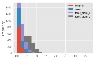
plt.figure()
data.plot.hist(alpha=1, stacked=True, bins=20)
plt.show()
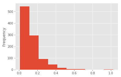
data['volume'].plot.hist(bins=10)
plt.show()
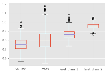
data.plot.box()
plt.show()
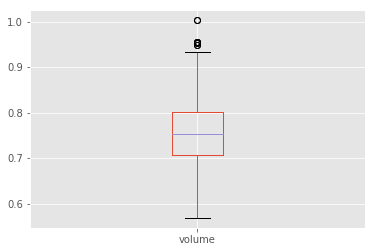
data['volume'].plot.box()
plt.show()
There are MANY tools I did not cover in this tutorial but this should show the basic building blocks of data analysis with Python. Here is an extensive cheat sheet from Hitesh Jethva of PCWDLD to aid you in the learning process. Feel free to comment below in case of any questions!